Introduction

HATS Chrom (HC) is an IDL (Interactive Data Language) – based application designed to process chromatographic data from multichannel instruments of Halocarbons and other Atmospheric Trace Species (HATS) group of the Climate Monitoring and Diagnostics Laboratory (CMDL) of NOAA, Boulder, CO.

HC is a standalone, fully independent IDL widget application; however, HC requires IDL to run. A compiled runtime version may become available should a demand develop. Multiple instances of HC are allowed to run simultaneously within the same IDL session, and they do not interfere with the command line operation in IDL. HC is fully portable between platforms and was tested on Unix, Windows and Macintosh. At the time of this writing, Macintosh showed the highest performance in visualization, while actual data processing speed is comparable for all tested platforms. HC was written in IDL v. 5.2 – 5.5; however, the original design may be updated at a later date to use more advanced features of upcoming versions of IDL.

No data is routinely shared by HC during a session. However, manual examination of the data and all relevant session variables is possible by restoring the saved files at the main IDL program level. Files saved by HC are standard IDL .sav files, and extensions used by HC (such as .flt, .cfg etc.) are used only for the easy identification of files by HC.

HC can be operated in two distinct modes: CONFIG and CHROM. CONFIG mode allows to define the chromatographic experiment parameters, such as molecules for each chromatographic channel, expected molecules peak edges and retention times, initial smoothing parameters, etc. (see HATS chrom CONFIG mode. section for more details). CHROM mode allows to proceed with actual integration of the peaks, using a peak edge detection method from an array of choices. Since HC is designed to operate on fast, highly compressed chromatography specific to airborne instruments, it incorporates tangent matching routines for locating peak edges and removing baseline effects. All peak detection routines are fully modular, i.e. new routines can be written from a template, and HC will recognize them using a naming convention and include them in future runs (see HATS chrom CHROM mode section for details). CHROM mode also has sub-modes for visual and quantitative quality control over the entire time series of injections for the whole (flight) experiment.

Starting chromatographic data processing in HATS chrom

Every chromatographic data processing experiment in HC starts from loading the chromatographic data. HC can not even start unless the data is loaded; this is because too many safety features would be required to keep HC from crashing when operating on an invalid data set. The original design of HC is to work with .itx files native to IGOR Pro for the Macintosh or PC. However, any other format can be used with a loading procedure that places the data in the appropriate format (see DATA specifications in the Appendix). Besides the data, HC relies upon the configuration information saved as fields in CONFIG structure (see CONFIG specifications in the Appendix). Loading routine needs to create these fields, or a configuration file needs to be present to start an experiment. The default file is “hc_default.cfg” (other, user-named .cfg files, may be used). HC has the capability to start up without the configuration file, in which case configuration is reset to default values and the operator needs to thoroughly set up every parameter to be used later.

To start HC, type “hatschrom” in the IDL command line. Alternatively, to open an existing experiment, type “hatschrom, ‘filename’ ” in the IDL command line. If HC does not find appropriate files it needs to initialize, you will be prompted to locate the files on the disk. During the startup with no pre-existing experiment, you will be asked to load .itx files, from which HC will determine the number of chromatographic channels, injection times, pressures, temperatures and other relevant information about your new chromatographic experiment. This step will be skipped if you are opening an existing experiment. After the loading of the data, you will be brought into CONFIG mode that will allow you to verify that the current settings are appropriate for your experiment.

HATS chrom CONFIG mode.

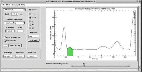
HC CONFIG mode (HCCM) is used for setting up the main experiment properties. HCCM (like all other modes) consists of two main panels: controls and plotting area. The controls allow to change the settings of the experiment, while plot area reflects the current state of the settings. Below the controls and their effects are described in details:

Channel selector. The number of channels in an experiment is determined from the loaded data. Number of channels can not be changed unless the data changes, for which new .itx files need to be loaded and current experiment will be lost. Choosing a channel causes an update to the rest of controls and to the plotting area, but the expected results will only be displayed if present CONFIG structure is already defined. If starting with no CONFIG file, all parameters will be set to meaningless values and will require setup.

Shift, s. This field allows to specify the shift of chromatograms for the current channel, in seconds, and is used for “unfolding” stacked chromatograms used on the fast airborne instruments. For standard chromatograms, this field needs not be changed and contains zero.

Smoothing parameters (Method, Width, s and Order). These is the setting for the initial smoothing of chromatograms. Smoothing can be specified individually for each channel. If a field is not used by a method chosen (for instance, “order” is not used by “boxcar”) then contents of that field are ignored.

B-Subtr. This field is molecule-specific, i.e. it only has effect on the currently activated molecule. Setting the checkbox will force HC to perform baseline subtraction, using zero air injections, before integrating that molecule peaks. Baseline subtraction performed at integration time and original chromatograms are not altered, so no particular processing sequence needs to be maintained.

Concatenate. Checking this box activates a button underneath it and allows to append together several current channel’s chromatograms. The number of chromatograms to be spliced is specified in a text field below. This is needed on the instruments that have channels that are longer than other channels. To use concatenation, set the chromatogram slider to the first valid sub-chromatogram of a “long” channel and check the box. Then, press the “Start concat at …” button; this makes the concatenation to start from either even or odd chromatogram. Make sure that the number of chromatograms per one “long” chromatogram is set to 2 (or other correct number), and change it accordingly when needed. Changing the number of chromatograms per long channel is allowed only the first time the Concatenate check box is activated for a given channel, so in order to alter this number, uncheck the box and check it again.

Start concat at… sets the beginning of concatenation of the “multiple-length” chromatograms, depending on what is the first “good” chromatogram number is.

Molecules radio buttons. This control allows to select the molecule for which the configuration parameters are being set up. Only one molecule at a time can be selected.

Add new molecule entry field allows to add molecule (abbreviated name) to the molecule list. This is useful when modifying the chromatography of a channel. Note that number of channels can not be determined by the user – it is obtained from .itx files. Adding a molecule to a list resets the molecule-specific parameters, such as B-Subtr or peak edges.

Kill mol button allows to delete currently selected molecule from the list of molecules for that channel. Killing a molecule results in resetting al molecule-specific parameters, so everything needs to be re-specified after number of molecules changes.

Left Edge entry field allows to manually enter the time in seconds from the beginning of the chromatogram at which currently selected peak begins. This value is used by tangent matching routines. The value in the field changes as active molecule changes, reflecting the molecule-specific value. Left edge can be set using the mouse by clicking the left mouse button (the only button on Macintosh) on the plot area in the desired location. Setting left edge using the mouse is insensitive to the vertical position of the mouse cursor. Green filling will appear on the plot area showing currently selected peak location (but only if all three entry fields, Left, Retention, and Right, are valid). It is recommended to set this value using a chromatogram from the middle of the injection series.

Retention data entry field shows the time in seconds from the beginning of the chromatogram when the crest of the peak of interest occurs. It can be typed in or entered using the mouse, by clicking the middle button of a three-button mouse, Option-clicking on Macintosh or Ctrl-clicking on a two-button mouse at the desired location on the plot area. It is recommended to set this value using a chromatogram from the middle of the injection series.

Right Edge data entry field is analogous to the other two. It can be typed in or entered using right mouse button or Command-clicking on Macintosh. It is recommended to set this value using a chromatogram from the middle of the injection series.

Plot area in HCCM is a window with a white background where the chromatogram is displayed. Plot area in HCCM displays chromatograms according to the channel and injection of choice (see “Current chromatogram” below). Plot area also will have a green shaded are that depicts the position and limits of the currently selected peak of interest. Zooming is supported by click-and-dragging the mouse cursor in HCCM; red zooming rectangle is drawn as the mouse cursor is moved. Multiple zoom-ins are supported. Gradual zoom-outs are not supported as unnecessary; full zoom-out is achieved by single-clicking the mouse to the left of Y-axis. Changing a channel causes automatic full zoom-out. Title at the top of the plot area in HCCM displays current chromatogram number, Stream Select Valve position and Flag information[1], injection pressure and temperature. It is possible that green filling of a peak may extend past the top of a plot in zoom-in mode; this is normal.

Current chromatogram slider allows to select the chromatogram of interest from the loaded dataset. It is recommended to use a chromatogram from the middle of the injection series when setting data processing parameters. On a zoomed-in plot, the scale will be preserved when moving from one chromatogram to another, therefore it is possible that chromatogram might fully disappear from the plot area. In this case, use full zoom out (see above) to view the chromatogram. Notice also that in this release, for concatenated channels, moving forward by pressing an arrow on the slider is not possible, because immediately subsequent chrom numbers are nonexistent. To move forward, drag the slider itself to desired position.

HATS chrom CHROM mode

HATS chrom CHROM mode (HCCrM) is utilized to perform the actual processing of the chromatograms. HCCrM actually includes several sub-modes – Integration, Set PED, Plots and Finalize. Integration allows to analyze peaks if peak detection is well-designed for the current chromatography. Set PED is related to CONFIG mode in that it writes into CONFIG structure which is saved from session to session for repeated application. It is separated from the CONFIG mode because it may need to be changed much more frequently than any other CONFIG mode settings. Plots mode allows plotting of time series and correlation plots for integration quality control. Finalize mode is for normalization of chromatograms before they can be used for post processing and creation of data submission files and plots. Below all the controls of the HCCrM are discussed in details.

Features of CHROM mode that are common for all three sub-modes are the following:

Channel selector works the same way as in HCCM and allows to select, which channel chromatograms are VISUALIZED at this time. Note that channel selector DOES NOT restrict the integration routines from processing peaks not currently displayed, should they happen to be selected as Active (see below). The only safeguard implemented is that peak limits will not be altered by clicking a mouse button for an active peak not currently displayed.

Subset (Cal, Air, All, etc.) specifies what subset of chromatograms will be used for integration following peak edge detection (PED). Default is ALL. Each subset can use its own set of peak edge detection parameters. This feature allows, for example, to use different methods of PED for zero air injections and other injections. In Plots sub-mode, this control changes from radio buttons to checkboxes, allowing more than one subset be plotted. In Integration and Methods sub-modes, this control is radio buttons to allow only one subset to be processed at a time.

Integrate / Set PED / Plots / Finalize pulldown menu allows to toggle between sub-modes. The sub-modes are discussed in more detail below.

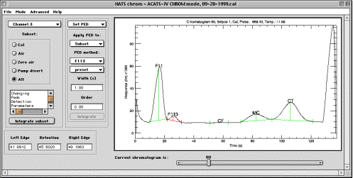
Integrate sub-mode

Integrate sub-mode allows fast batch processing of chromatograms. This is valuable in case the chromatography is well-understood and peak edge detection methods are skillfully set for subsets of chromatograms and produce good results.

Information window. This window, located just below the Subset control, displays information about the PED parameters of a molecule which checkbox the mouse cursor last passed over. To display information on current subset PED, place cursor over the molecule of interest checkbox.

Integrate subset button starts processing of the current subset using its PED parameters. Integration will be performed for all active molecules (those which checkboxes are checked).

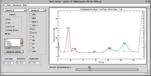
Active molecules checkboxes set the molecules on which to perform PED and integration. PED and integration are performed seamlessly in one operation. However, if PED fails, integration produces unpredicted results. Refer to Plots sub-mode below for quality control. The peak displayed in red is active peak, for which edge and retention setting is available using mouse cursor. This peak is the uppermost currently selected checkbox.

Plot area in the Integrate sub-mode is similar to described in Config Mode section above. Peak filling is not displayed, instead peak edges and retention are displayed according to the current settings (which are –10.0, if no PED has been performed yet, and no peaks are displayed at all). Peaks are labeled with molecule definitions. Zooming is performed in the same exact way as in CONFIG mode. Besides zooming, plot window allows interactive definition of peak edges and retention time for the uppermost selected Active Molecule checkbox of the currently displayed chromatogram, shown in red on the plot. Use left mouse button to set left edge, middle button for retention and right button for right peak edge. If any peak parameters are changed interactively, integration is immediately performed and area-hight are updated for that peak. If the currently active molecule has baseline subtraction turned on, then the color of the chromatogram in the plot area becomes dark blue, and reflects the shape of the chromatogram with baseline subtraction (zero air subtraction). Once a molecule becomes active that does not use baseline subtraction option, the chromatogram again becomes black and returns to the normal scale. Notice that there is another, thin grey chromatogram in the plot area that shows the original chromatogram before the smoothing was applied.

Current chromatogram slider acts as described in HATS chrom CONFIG mode above, scrolling through available chromatograms.

Left edge, Retention, Right edge. These fields allow typing and will set peak parameters for the uppermost selected molecule of the current chromatogram.

Set PED sub-mode.

This sub-mode sets fields in CONFIG structure that define the way chromatograms will be processed in the currently active subset. This sub-mode also serves as a testbed for PED methods that either can be assigned to a subset or have been newly developed. Refer to the discussion of Channel selector and Subset radio buttons on page 6.

Information window is inactive in Set PED sub-mode.

Integrate subset button starts processing of the current subset for the molecule currently selected in PED panel. Note that in Set PED sub-mode, only molecule set in PED panel will be processed, even if other molecules were previously selected in the Integrate sub-mode.

Apply PED to: droplist. This droplist selects the target for peak edge detection and integration, which may be the entire subset or only current chromatogram. If the target is “Current”, the pushbutton will become available at the bottom of the PED panel to integrate current chromatogram. If the target is “Subset”, then using controls below will set the method fields in CONFIG structure for the molecule and subset of choice.

PED method controls. These include Molecule and Method droplists which serve for selecting active molecule and assigning PED method to it. Molecule droplist does not perform any action, and only indicates what molecule is used to set PED parameters. Method droplist sets the method for the subset (if Apply PED to: droplist is set to “Subset”). Note that is the target is set to “Current”, no method in CONFIG will be changed.

Molecule: use this droplist to select target molecule for setting PED method or integration.

Method: use this droplist to select PED method for the selected molecule.

Width (s) and Order fields pass the integration parameters to currently active PED method. Not every PED method will use them. If the target for PED is “Subset”, entering a number in this fields will set the fields in CONFIG structure and they will be saved in the experiment file. If the target is “Current”, values entered are not preserved. To force them to be saved for the subset, choose “Subset” as a target, re-select the method, place focus into Width and Order fields and press “Enter”. When in “Integrate” sub-mode, the values currently stored in CONFIG will be displayed in the information window.

Integr. #… pushbutton only becomes available when the “Apply PED to:” droplist is set to “Current”. The number on the pushbutton indicates current chromatogram. Pressing the button causes the selected peak to be integrated using currently selected method. This is useful when attempting to find the best method for detecting a certain peak, because the method is not applied to the subset so processing time is minimal. Results of the integration become immediately visible in the plot area in the form of peak edges and baseline.

Plot area in Set PED sub-mode is identical to described in the “Integrate” sub-mode section. Peak edges and retention are displayed according to the current settings (which default to peak edges set in CONFIG mode, if no PED has been performed yet). Zooming and interactive definition of peak edges and retention time for the molecule selected in the PED panel, for the currently displayed chromatogram. Use left mouse button to set left edge, middle button for retention and right button for right peak edge. If any peak parameters are changed interactively, integration is immediately performed for that peak.

Left edge, Retention, Right edge. These fields allow typing and will set peak parameters for the uppermost selected molecule (not necessarily displayed!) of the current chromatogram.

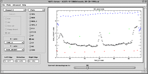
Plots sub-mode

All controls in this sub-mode are similar to described in “Integrate” sub-mode on page 7. The difference is that Information window in Plots sub-mode is replaced with the droplists for choosing variables to be displayed on X and Y axes. Subset chooser is not available in this sub-mode because all subsets are displayed using color coding. If a large number of subsets is present, colors may be recycled as only 4 colors are defined in the code.

Channel selector and Subset selector are not available in this mode because molecule choice is sufficient for defining the contents of plotting area.

X-axis and Y-axis droplists select variables to be placed on the corresponding axis. The results of choosing are immediately displayed in the plot area. Note that these droplists are updated every time the user chooses “Plots” sub-mode. Therefore, if a new type of response is calculated for the molecules (width of a Gaussian fit, for example), then this field will become available for displaying in Plots sub-mode.

Plot area in Plots sub-mode is used for identifying the chromatograms. Left-mouse-click on a point of a correlation plot will position the Current chromatogram slider underneath the plot area to the number of that chromatogram. Right-mouse-click on a point of a plot will immediately bring up that chromatogram in the Set PED sub-mode targeted for that channel, molecule and chromatogram number for detailed analyses, allowing either fine-tuning of PED parameters or simply manual integration of the peak. Zooming is available in the usual way.

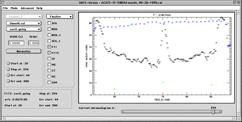
Finalize sub-mode

This sub-mode allows to normalize processed data using in-flight calibration gas measurements and prepare the data for post processing (preparation of data submit files). The reason post processing is detached from chromatogram processing is sometimes calibration values on cal cylinders are updated, which causes the need to apply correction to entire missions worth of data at a time. Instead of altering a lot of flight experiments, only one post processing experiment will need to be revised in such case.

Controls completely change in this sub-mode. Channel control is irrelevant because all molecules are displayed at the same time. Multiple molecules can be selected, but only the to post one will be displayed. The display is provided using the coordinate axes chosen in the Plots mode.

Display panel contains the plot of the molecule and allows zooming similarly to other modes of operation. In addition, manual quality control can be performed on the plot. That is, obvious outliers or points known to be problematic for some reason can be removed from the data processing. This is accomplished by using middle mouse button (or Control-drag with a 2-button mouse, or Option-mouse drag on Macintosh) that allows to draw an arbitrary area in the display window. All data points inside that window will be eliminated and immediately disappear from the screen.

It is recommended that data elimination, especially if calibration points are removed, is performed on the _RAW data. This way, changes will be automatically reflected in the normalized dataset. It is, however, possible to alter _NORM data as well, if desired.

Smooth cal / Fit cal droplist allows to select a method for preparing calibration injections for interpolation. At the time of this writing, only smoothing was available and using this control has no effect.

Smoothing method droplist defines the method used to smooth the in-flight calibration before interpolation. Traditionally, for the ACATS-IV data processing the calibration was smoothed instead of fitting, and RMS of the residuals from smoothing was included into the estimated error of measurements.

Width and Order fields are identical to such described earlier for smoothing methods.

Normalize pushbutton is used to perform normalization and store the results in PROCESS structure. See description of PROCESS in Appendix for details.

Start at, Stop at, Err start, Err stop radio buttons are used to specify data processing intervals for the currently selected molecules. Place the Current chromatogram slider at the desired location and press the radio button to set its value. The label of the button will change reflecting the selection. Note that buttons immediately release after setting their values. Note that the labels of radio buttons keep track of whether the processing limits of selected molecules are the same or not. If all active molecules have the same limits, labels display those limits. If a molecule(s) in the active set have different parameters, the labels will have “diff” appended instead of processing information. This does not interfere with simultaneous normalization of molecules whose limits were defined differently.

Active molecules checkboxes indicate which molecules are going to be affected by using other controls. The uppermost selected molecule will be displayed in the plot area according to the last choice of X and Y variables in Plots sub-mode.

Information panel contains the smoothing and processing information for the molecule which checkbox was last visited by the mouse cursor. To display information about a molecule, place cursor over its checkbox.

Menus, Advanced use and Development

Menus

Menus available in HATS Chrom are mostly self explanatory and require few comments. Some details worth mentioning are as follows:

-       There is no warning if a user modified an experiment and then quits without saving changes.

-       Save Experiment control actually functions as “Save As” control, i.e. an option to alter file name is always offered.

MODE menu chooses whether HC is in CONFIG or CHROM mode. CONFIG choice also allows to Edit CONFIG, which brings the user into CONFIG mode of HC, Save CONFIG for future use as a user-named file or save default config file, “hc_default.cfg”, to be used in future experiments. Note that every experiment has integrated CONFIG in it, regardless of whether or not CONFIG has been saved separately.

ADVANCED menu of HATS Chrom allows some non-routine operations that are helpful in defining how experiments are processed. In particular, it contains such important choices as Instrument definition and Flag definition.

Instrument menu choice allows setting the name of the instrument in CONFIG structure that identifies which instrument performed data acquisition. The name of the instrument also appears on the title bar of HATS chrom experiment.

Define FLAGs is a choice available under Advanced menu. This control should be used in CONFIG mode if CONFIG is not loaded at the beginning of experiment and the user is setting up the entirely new configuration. This control brings up a table that contains all choices of chromatogram flagging available from the data: SSV positions and Flags. Remember that all those need to be produced by the loading routine. Then, the user can define the meanings of those choices, like “Selpos 1: Cal”, “Selpos 2: Air”, etc. The definitions provided by the user are later incorporated into the subset chooser in CHROM mode.

Use Eng. Data function is not implemented in this release.

Reset PROCESS menu choice allows to reset all contents of processed experiment to initial blank values. This is useful in case you suspect data processing is going wrong due to a bug. Otherwise, you need not reset the processing, because simple re-integration will overwrite previous values in PROCESS structure.

Naming conventions

Naming conventions in HC are used to allow easy expansion of HC without the need for detailed understanding of full HC functionality. The following naming conventions are used by HC:

hc_sm_*: these files are assumed to contain smoothing functions. Template for smoothing routine is provided in the file “hc_template_sm.pro”. At the beginning of each session, HC searches for “hc_sm_*” compiled functions and uses their names to define the list of available smoothing methods in CONFIG and CHROM:Finalize modes.

hc_ped_*: these files are assumed to contain Peak Edge Detection routines. At the beginning of each session, HC searches for “hc_ped_*” compiled functions and uses their names to define the list of available PED routines for CHROM:PED method mode.

Other naming conventions are internal (“RAW_”, “NORM_”) and should be considered when writing more in-depth extensions to HATS Chrom, for instance other peak assessment methods than height and area. See the discussion of these in Appendix, Process structure and below, in Normalizing flight data section.

Templates

HC is designed to be modular, so that a user can develop some key routines and use them in HC without modifying the core of the program (see Naming Conventions above). For each naming convention, a template is provided that has pre-coded basic operations for that type of routine. Templates by themselves are not functional at all, although are designed to compile. All the user then needs is to add custom processing and rename the routine to give it a meaningful name, following the convention. Next time HC starts, it will locate the new routine and make it available for data processing. Templates themselves follow a simple naming convention: “hc_template_*.pro”.

Same philosophy is useful when data source is changed from .ITX files to some other format. HC has no preference over what routine supplies the data for it. However, at the time of this writing no indication existed that other format needs to be made readable. Therefore, loading is handled by “hc_itx.pro” routine, which is called from “hatschrom.pro” directly. To use a custom routine for data loading, make sure that routine creates the appropriate format for the DATA and CONFIG structures (see Appendix for details).

Normalizing flight data

Normalizing flight data is performed using smoothed or fitted in-flight calibration. In this release, two methods of assessing chromatographic peaks are provided – peak height and area. Most of the time peak height gives higher precision. However, other approaches are anticipated such as, for instance, evaluating the width of a gaussian fit to a peak. To implement such thing, one needs to alter PROCESS structure (see Appendix). Following naming convention of having RAW_ and NORM_ fields in PROCESS , add these fields to PROCESS using HC_STRUCT_UPDATE function. Then, do the same to the contents of the PROCESS.PRECISION array. Once these variables contain new NORM_* fields, they will be automatically recognized and made available for post processing by the post processing software.

 

NOTE -> It is possible to have multiple versions of the same flight data open as several HC experiments at the same time. This way, different data processing methods can easily be compared. Once the .flt file located on a hard disk was opened in HC, it is no longer used by HC (of course, it can be overwritten by File Save operation). Another HC experiment may be opened from the same saved file. If neither HC experiment is saved, the original file will not change at all.

Hats Chrom Calibration Curves

Hats Chrom has integral mechanism for gas chromatograph calibration processing. Calibration is different form the rest of HC in that it is object-based. This means that calibration curves in are not enclosed in a special application or experiment, like, for example, flight data. HC calibration curves are independent IDL variables that contain the initial calibration experiment data, calibration tank assignment, mixing ratios for tanks and routines necessary for creation, application and precision estimation. This distinction is rather technical but important for the user in that no memorization is needed when applying cal curves, and no generated curves are stored anywhere. Calibration equations are created by appropriate routines on demand.

HC calibration curves are represented by IDL object class called “hc_calcurve”. See Appendix, HC_CALCURVE, for technical details about hc_calcurve object and its methods. Graphical interfaces are provided for convenience of creating, modifying and applying a calibration curve.

Creating a new calibration curve: reading data

Creating calibration curves is easiest from the HATSchrom experiment that contains the integrated calibration chromatograms. Create a calibration by choosing “Calibration” from the “Advanced” menu. Once the calibration curve GUI appears, it is no longer linked to the HATSchrom experiment, which can be closed, if desired. It is recommended that calibration curves be created using GUI.

Alternatively, cal curve object can be created manually. To create a new calibration curve, you need to have a processed calibration experiment first (i.e., integrated chromatograms). Then, create a calibration curve by calling IDL statement such as

CC = obj_new(’hc_calcurve’, file=’01-22-2000.cal’, tank_values=’tanks.csv’)

where file keyword is set to the name of calibration HC .sav file, and tank_values is set to the name of the file containing the list of calibration tanks in comma separated format (this file is typically provided with HC). CC is now a calibration curve object. It can be manipulated inside the IDL development environment absolutely independently of any other HC application.

NOTE -> If a calibration curve has never been created in the current IDL session and is being used in post processing experiment, IDL will not auto-compile the calibration curve processing code. Make sure that either the binary file was used to start HC, or the entire HC library was compiled first.

New curve can also be created in steps, without initializing the data at the time of object creation, using common IDL syntax for object operation:

CC = obj_new(’hc_calcurve’)

CC -> setProperty, file=’01-22-2000.cal’

CC -> setProperty, tank_values=’tanks.csv’

Graphical user interface for tuning the calibration curve

Once the calibration has been initialized with the data, cal curve object needs assignment of calibration tank values before the curves can be generated. This step is accomplished through a GUI interface only, as IDL interactive control is too laborious. To activate GUI, execute the following (presuming the above introduced CC name for the cal curve object):

CC -> gui

Graphical interface is a standard window in the system-native format. Its title contains the date of the calibration experiment (derived from the chtomatogram source files). The GUI consists of two parts, controls and plot area. Plot area also allows at least three modes of interactive and sometimes irreversible data control, so be reasonable when clicking and dragging the mouse cursor in the plotting area. GUI operates in two modes, “Assign”, used for assigning calibration tank values to subsets of injections, and “Curve”, for fine tuning the calibration, deleting outliers and visualizing cal curves. All available controls and modes of operation are discussed in detail below.

All of the following controls are used within GUI only. When cal curves are used at a later time, GUI and its controls are not involved. However, from GUI they make irreversible changes to calibration curve data (the data can, of course, be reloaded, if a mistake was made; given high speed of reloading, no undo facility is provided).

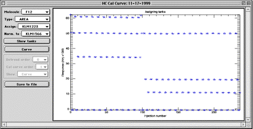
Molecule and Type droplists serve for choosing which molecule is currently being displayed and what particular peak assessment method is being used. Values of these controls are determined only by the fields available in a calibration experiments, and are loaded from the latter using NORM_* naming convention.

Assign droplist contains the list of all available calibration tanks loaded into the calibration curve object from the comma tank values separated file. Use this control to choose calibration cylinder that was used for a series of injections, displayed in the plotting area. Once the tank is selected, use plotting area controls to assign cylinder values to chromatogram index (see below). This control becomes unavailable in “Curve” mode. Notice also that there is no need to assign zero air to any injections, unless you have first by mistake assigned tank values to them. Gravimetric values of all injections default to zero, so any injection that was not assigned a tank value will have zero mixing ratio (“zero air”).

Norm. to droplist also contains the list of calibration cylinders. Make sure this control is set to the cylinder that was used to normalize the flight experiment that the cal curve is intended to be used for.

Show tanks pushbutton brings up a plot showing relative positions of calibration tanks, for the molecule of interest. This is useful when assigning tank values to groups of injections.

Curve / Assign pushbutton is used to switch between the two modes of operation of the cal curve GUI. Press the button to toggle to the mode which name is currently displayed on the button. For instance, if the button displays “Curve”, it means you are presently in “Assign” mode.

The following controls only become available in “Curve” mode.

Detrend order droplist allows to select the order of a polynomial fit, which is used to de-trend the cal curve dataset using the normalizing cylinder data. In the example above, this data is seen at about 50 kHz as a horizontally arranged line of data points. Orders for de-trending are hard coded in the method function. Zero order is no de-trending. Order of 1 is linear fit. Higher orders can be used for polynomial fitting. Typically, second order provides optimal detrending; however, higher order may be needed for some unstable calibration experiments. Experiment with detrending orders while displaying the residuals from normalization (“N. resid.”), and choose the lowest order providing satisfactory residuals. The optimal detrend method will be memorized in the cal object, because it is to a degree a property of the data in the object. It is unnecessary to burden the user with memorizing detrend orders that have once been found optimal.

Cal curve order droplist allows to select the order of calibration curve to visualize. Remember that this is for visual quality control only, and has no effect at all on the order of cal curve later applied to a Hats Chrom experiment. Order can be from 1 to 4 and is hard-coded into the function. Should it be necessary, higher orders may be entered easily.

Show droplist allows to choose the data to be displayed in the plot area. The choices offered by this control are “Curve”, “N. resid.” And “CC. resid.”. If “Curve” is selected, calibration curve is displayed for the current selection of controls (F12, Area, Normalized to KLM1566 in the example above, detrended according to Detrend order control and fitted with a polynomial of the Cal curve order). If “N. resid.” is selected, the residuals from de-trending the normalizing calibration cylinder data are displayed in the plot area. If “CC. resid.” is selected, the residuals from the calibration curve fit are displayed. The latter two regimes are convenient for eliminating the outlier points and creating more compact data to be fitted for calibration.

Plot area controls are mouse actions performed inside plotting area. There are three actions available using the mouse. Left-mouse-drag results in the appearance of a green rectangle and is used for zooming in inside the plot area. Zooming is identical to that in HC, i.e. zoom-out is full and is achieved by clicking to the left of the left Y axis inside the plot area. Middle-mouse-drag in the plot window results in the appearance of a red rectangle. In any mode of operation, any data points that fall inside the red rectangle will be permanently deleted from the calibration. The change will only affect the current molecule and type, e.g. “F12 Area” on the example picture above. Since this action can not be undone unless the data are reloaded, caution needs to be exercised. If you have started dragging and discover, to your dismay, that a red rectangle appeared instead of green or blue, do not panic: just move the cursor such that no points are encompassed by the rectangle, and release the mouse button. The database in the cal curve object will remain unaltered. Deleting points may cause “floating point errors”, which, although annoying, appear to cause no problems for functionality. Right-mouse-drag (blue rectangle) in the plot window at the time of this writing is only effective in “Assign” mode, and has no effect in “Curve” mode. In “Assign” mode, use right mouse button to encompass a group of points that have the same source gas (cal tank number) injected during calibration. On the example above, each of horizontal data lines is the result of repeated injections of the same calibration standard. Thus, to assign a tank to a group of points, first select the tank ID from the “Assign” droplist, then use right mouse button to draw a blue rectangle around the points you want to assign that tank to. This procedure is fully reversible, i.e. tanks can be re-assigned as necessary as many times as necessary.

Save to file button allows to save the calibration object to a named file. File name defaults to the date of calibration with .cc extension.

Fine-tuning a calibration

Once the data are loaded, tanks are assigned and cal curves are available for visual inspection, calibration curve object can be fine-tuned to produce the best fits possible from the data it contains. Usually, detrending and measurements are not perfect and noise will be present in the response versus gravimetric value chart. It is recommended that outliers be removed from the calibration, because they affect the precision of a polynomial fit much more than they reflect actual imprecision of the measurements. It is recommended to delete (using “red rectangle”) those points for each molecule that fall far apart from the rest of the data. “CC. resid.” Display is especially convenient for this task, because outliers can be easily seen as points with unreasonably large residuals. Use “red rectangle” to delete the outliers. Cal curve object will be modified and any future curves generated from is will not be affected by deleted outliers. Remember that cal curve object needs to be saved to file before its updated contents will have any effect on the post processing of the flight data.

Creating a calibration curve from an HC experiment

For convenience and seamless operation, creating a calibration curve can be initiated from the inside of an HC experiment. However, not doing so does not cause any problems, as cal curve objects are fully independent, and can be created at any time interactively. From HC experiment, once a cal curve object has been created, its further development will be accomplished through the use of the calcurve GUI (see above), which will appear once the data is loaded from HC experiment. To create a cal curve object from inside an experiment, use the “Calibration” choice from “Advanced” menu.

Post Processing of the data

Post processing involves applying calibration curves to the chosen normalized peak data from a flight experiment (i.e., Area, Height, etc.). Post processing is separated from the flight processing to allow easy alterations to final data set in case of a calibration scale changes or appearance of data outliers. Post processing stores no data in its experiments, and extracts normalized descriptor fields from the flight experiments as it needs them for processing. Post processing in HATSchrom is organized in such order that changes to either calibration curves or flight experiments can be made while PostProc is active and open. Post processing simply catalogs the flight experiments and calibration curves and allows the user to assign the calibration dates, polynomial fit orders, de-trending (normalization) fit orders to each molecule in each flight experiment, so that this information does not need to be re-entered to produce exchange files at a later date.

Post processing can be initiated from the “Advanced” HATSchrom menu by choosing “Post processing”, or by typing:

POSTPROC

on the IDL command line. Optionally, name of post processing experiment can be supplied, as follows:

POSTPROC, ‘Solve_postproc.pp’

If no file name was provided, PostProc will offer the user to locate a file. If user cancels the locate file dialog, PostProcessing will create a new post processing experiment by cataloging the flight (“.flt”) and calibration curve (“.cc”) files that it was able to locate in the current directory. If it finds no useful files, it will prompt the user to locate the directory containing the flight data. All calibration curve assignments in a new experiment default to the alphabetically first calibration curve date, Height response type, second order calibration curve and second order detrending fit. As it is changed by the user to reflect the proper calibration for individual flight dates, these new settings will be preserved when the new experiment is saved, and restored automatically the next time that experiment is opened.

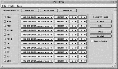
Controls in Post Proc include menus, radio buttons, droplists and pushbuttons.

Menu controls are mostly self-explanatory. File menu allows to save the current settings into a file or exit, in which case a warning is given if the work was not saved. Use Flight menu to choose which flight to post process.

Tools menu, Export to variabe menu option. Allows to process flight data, but instead of writing the result into an exchange file it will be output into an IDL variable at the main IDL session level as a pointer. When the user chooses “Export to variable”, PostProc will process flight data exactly as it would do it to make exchange files, but will redirect data output into a temporary storage location. Menu choice will change to “Stop exporting”. Once the data needed are processed, choose “Stop exporting” menu option. This will bring up a dialog window, where the user can type the name of IDL main level variable to receive the data. If the variable exists, it will be overwritten, otherwise it will be created. Only mixing ratios will be stored, and no header that is standard in exchange files will be created. Data in the varaible are in the form of a 2D array with the first row consisting of injection time stamps as Julian date. The rest of the array are mixing ratios ordered the same as molecule names for all channels.

Flight label in the upper left hand corner indicates which flight is currently being processed. It may also change to “C-CURVE MODE” indicating that curve editing mode is active and no changes are being made to the flight data processing settings.

Show mol. button is used to display a time series of the chosen molecule’s mixing ratios, using currently selected calibration curve, data type and fitting parameters.

Write file button control makes an exchange file using all molecules’ settings for the current flight. The following needs to be considered. Molecule names are neither being read nor written from a HC experiment. The list of molecules in the exchange file is recorded in the file named “gc_header.txt” which will be read before the exchange file is created. Make sure that the list of molecules in “gc_header.txt” is in the right order and current.

Write all button will loop through all flights in the list and make exchange files, or, if Export to variable was used, store all flights data into an IDL variable.

Molecule choice radio buttons. The number of these may vary according to the molecule presence in the HC file. The currently selected molecule is the one which calibration curve can be displayed or edited, and which mixing ratios can be displayed by pressing Show mol. pushbutton. Molecule selection has no effect on the creating of the exchange file, where mixing ratios of all molecules are always calculated.

Calibration parameters chooser. This multi-droplist section defines the set of calibration parameters used for each molecule for the currently chosen flight date. The choices are calibration curve name (typically meaning the date), parameter to be used (Area, Height, etc – if available), normalization fit order and calibration curve fit order. These parameters are remembered for each flight and are saved when File-Save menu is activated.

C_CURVE MODE panel contains the set of controls that allow immediate access to calibration curves directly from Post Proc experiment.

Start-(Stop) button (de)activates the ability of calibration parameter controls to alter the settings for molecule processing. Pressing Start causes Flight label to change to “C-CURVE MODE”. When in this mode, choosing a molecule’s parameters will not be remembered and saved. This way, it is easy to visualize different calibration curves (see below) without going back and re-setting all previous parameters. To return to processing of the data, press Stop and all settings for flight processing will be restored. Start-Stop is useful for Plot and O-plot functionality (see below).

Edit pushbutton will display the calibration curve object for the currently selected molecule in its own GUI, allowing calibration changes. This is useful if there appears to be a problem with outliers in a calibration curve. Through CalCurve GUI, these may be immediately alleviated, cal curve saved and Post Processing will resume with the updated calibration data.

Plot pushbutton will display calibration curve for the currently active molecule, data type and fitting parameters using the Display procedure. Display allows zooming, legends, color changes etc.

O-plot button appends calibration curves to a Display window created by Plot. This is useful for visually comparing calibration curves that use different fitting parameters.

NOTE -> It is important to remember that Post Proc is completely separated from the data at all times. This means that any flight or calibration can be modified at any time, whether a Post Proc experiment that uses that data is open or not. When Post Proc calculates mixing ratios, it will always restore saved data and calibration curve files from the disk prior to processing.

APPENDIX

Here, a technical discussion is provided for those who might wish to alter the core code of HATSchrom.

First, HC is not written as an object application. Historically it was because I was not familiar with IDL’s OOP quite well when I started. However, it turned out that in many aspects, HC data organization was laid out almost perfectly from the very beginning. Later, an attempt was made to convert HC to more structured, objectified application with Chrom, Peak and Flight objects forming a nice hierarchy. Despite the promising straightening of the code, this appears to have an important flaw: numerous objects tend to slow down IDL save operation, as well as many other operations that are optimized for vector processing in IDL.

Therefore, converting the data in HC to object (or even pointer) arrays is highly discouraged. Experiment save and restore time for those types of data organzation doubles, as does the required storage space. In contrast, replacing some repetitive, low volume elements of HC with objects seems to be a very good idea. Examples of these are Peak Edge Detection (PED) methods, Smoothing, Normalizing etc. If this is implemented, one might want to look into alternatives to saving object data because this slows down the otherwise fast disk operations. One of the ways allowing to save object information without saving object heap variables is to save object type and recreation parameters as a string (array).

I want to thank Dr. Eric A. Ray for introducing me to IDL. Many thanks to Mr. Geoffrey S. Dutton for maintaining and improving IGOR Pro code for peak edge detection using tangent fitting. Most of the design of HATSchrom was inherreted from the original design of NOAHchrom that was written in IGOR Pro and revised many times over the years. Drs. Dale F. Hurst and Fred L. Moore are thanked for their suggestions on improving peak detection and analyses, as well as laying out user-friendly graphical interface. Dr. James W. Elkins is thanked for his overall support.

This software was written as part of the University of Colorado research program funded by NOAA and NASA, and as such is subject to the laws and regulations of these institutions for the sale and distribution of software.